The last time I blogged about NXP’s sensor fusion
solution (Open-source sensor fusion) was almost a year ago. Since then, it’s been downloaded
roughly 2,000 times and we have a very active
NXP Sensor Fusion Community. I would like to thank everyone who has taken the time to check it
out. I would also like to invite you to download our new (Version 5.00)
release, posted just this month. Features of the new release include:

- New and improved 6-axis and 9-axis Kalman filters
- Addition of FRDM-K22F support for KDS
-
Additional “bonus” bare board projects for 3-axis tilt and
6-axis eCompass
-
Updated documentation, including data sheet, user guide and full details of
the Kalman algorithms
- All source code included under BSD 3-clause open source license
-
Community support at
NXP Community
An updated NXP Sensor Fusion Toolbox for Windows supporting all of the
above is also available. Make sure you download this at the same time
you get the library, as both have changed. New versions of
library/toolbox are not compatible with old versions of toolbox/library.
By far the biggest change the list above is the first bullet.
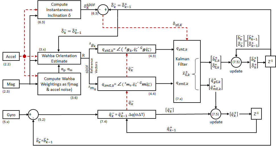
We’ve changed how the filters track linear acceleration and magnetic
interference. In the previous generation filters, we tracked these
explicitly as state variables for the system. In the new filters, we
treat them as noise and adjust weighting factors and co-variances based upon
how much acceleration and magnetic field differ from expected values.

We use those weighting factors within a least squares fit of
known vs measured gravity and magnetic vectors. This technique was
first proposed back in the 1960s by Grace Wahba as part of NASAs work in
determining satellite attitude as a function of observed versus known
star locations. Using this technique gives us a very elegant
way of automatically handling magnetic interference and effects of linear
acceleration by biasing our orientation estimate one way or
the other. From the computed orientation, we can extract new
estimates for gravity and magnetic field, which are then compared with
gyro-compensated estimates from the last iteration of the filter. Those
errors then become inputs to our Kalman filter. The overall process is
illustrated in the figure above. Not shown is the hard/soft iron
compensation step, which precedes the Wahba calculation.
Don’t worry if none of that makes sense right away. But if you
take the time to work through the math, you’ll find this figure will
act as a handy frame of reference. And when you try the new filters,
you’ll discover that they converge faster and are generally more
stable.
We only do “full web releases” on a periodic basis. Bug
reports and new features generally show up on the community site
first. Be sure to check in there before starting any new development.
Our BSD 3-clause open source license continues to apply, so you can
(still) quickly add unique features to your products without
worrying about pesky license restrictions.
Michael Stanley “works” on fun sensors and systems topics at
NXP.


