We have made a big push in recent years in the realm of
sensor fusion. We are very proud of those accomplishments, and
today we’re still the only major sensor vendor to take our
solution
fully open source. But you can do a whole lot more with sensors than simply modelling
motion. In his recent Embedded Beat blog posting, Ian Chen introduced the concept of
Sensor Data Analytics. Essentially, this boils down to
looking for patterns in raw sensor data, and their relationship to everyday
activities and events. The starting point for this is often raw vibration
data from an accelerometer. The machine condition monitoring industry
has been utilizing vibration data for many years to predict machine failure
before it occurs. If you’re looking online, you’ll find
the industry has a number of aliases:
All refer to essentially the same thing. For cost reasons, machine
monitoring was historically used only for very expensive machines that
cannot tolerate unscheduled downtime. MEMS technology has now reduced
the sensor cost to negligible levels, and the only thing standing in the way
of further adoption is expertise and software availability. And things
are changing there too.

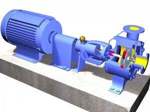
Figure 1: Centrifugal Pump (source:
http://en.wikipedia.org/wiki/File:Centrifugal_Pump-mod.jpg)
Let’s look at some examples. The figure above shows a
“classic” industrial application. A rotary motor is
coupled mechanically to a centrifugal pump. The motor, coupling and pump
are all subject to various physical problems. These include things like:
- shaft misalignment
- bearing failures
- load imbalance
- looseness
- gearbox faults
- drive belt failures
- resonance
Interestingly, ALL of these problems manifest themselves as changes in the
vibration signature(s) of the system.

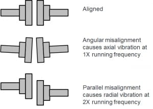
Figure 2: Shaft Misalignment
Figure 2 shows variations in shaft alignment between the motor and
pump. These can cause a 2X rotation frequency term to show up
in Fast Fourier Transform results run on vibration sensor outputs.

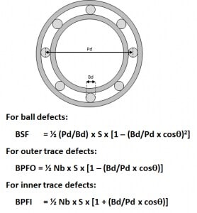
Figure 3: Effects of Bearing Defects
Figure 3 is a simplified view of a bearing, with inner trace, outer trace and
roller balls between the two. Defects in any of these three will
again manifest themselves in the vibration data FFT. The changes in
frequency content are well understood as a function of the bearing
geometry, and are shown n the figure. The variables in these equations
include:
- Pd = pitch diameter
- Bd = ball diameter
- Nb = number of balls
- S = speed (revolutions/sec)
- q = contact angle
- BSF = Ball Spin Frequency
- BPFO = Ball Pass Frequency of Outer Trace
- BPFI = Ball Pass Frequency of Inner Trace
In coming posts, I’m going to explore other patterns. Some
are deterministic (like those shown above). Others are purely
statistical. My colleagues and I will also give you a
peak at the tools and workflow we’re using to collect and analyze
data. This includes advanced machine learning techniques,
which is an area of science that didn’t even exist when I went to
school. We’re having a lot of fun using it to look for
patterns. You can too.
In the meantime, if you are intrigued by the examples shown above, pick up a
copy of the
Harris’ Shock and Vibration Handbook (Sixth Edition). Chapter 16 gives a great overview of “Condition Monitoring of
Machinery”.


